The detailed study of neural network weights

21 Feb, 2026

When considering the weights, we can consider an in-depth study that looks at the activation and gradient statistics. This is the central lesson from Karpathy. To treat your network as a scientific instrument. Measure what is happening inside it. The loss curve alone tells you almost nothing about the why.

I implemented the entire pipeline from scratch in NumPy, no PyTorch, to make sure every number is traceable. The code below builds a character-level MLP for name generation with multiple hidden layers and tanh activations, then studies what happens under two initialization regimes.

The experiment

The setup is a 5-layer MLP with 200 neurons per layer, trained on a small name dataset. We compare two scenarios: weights drawn from a standard normal $𝒩 (0, 1)$ (bad), and weights scaled by the Kaiming factor $\frac{gain}{\sqrt{n_{in}}}$ (good).

# BAD init, no scaling.
W = np.random.randn(fan_in, fan_out)

# GOOD init, Kaiming scaling for tanh.
gain = 5.0 / 3.0
W = np.random.randn(fan_in, fan_out) * (gain / np.sqrt(fan_in))

The gain of $5 / 3$ is the standard PyTorch value for tanh. The reasoning: tanh is a contractive function (it squishes its input), so you need a gain greater than 1 to compensate and keep the activation standard deviation roughly constant across layers.

Forward pass activations

The first diagnostic is to look at the distribution of activations at each layer after a single forward pass.

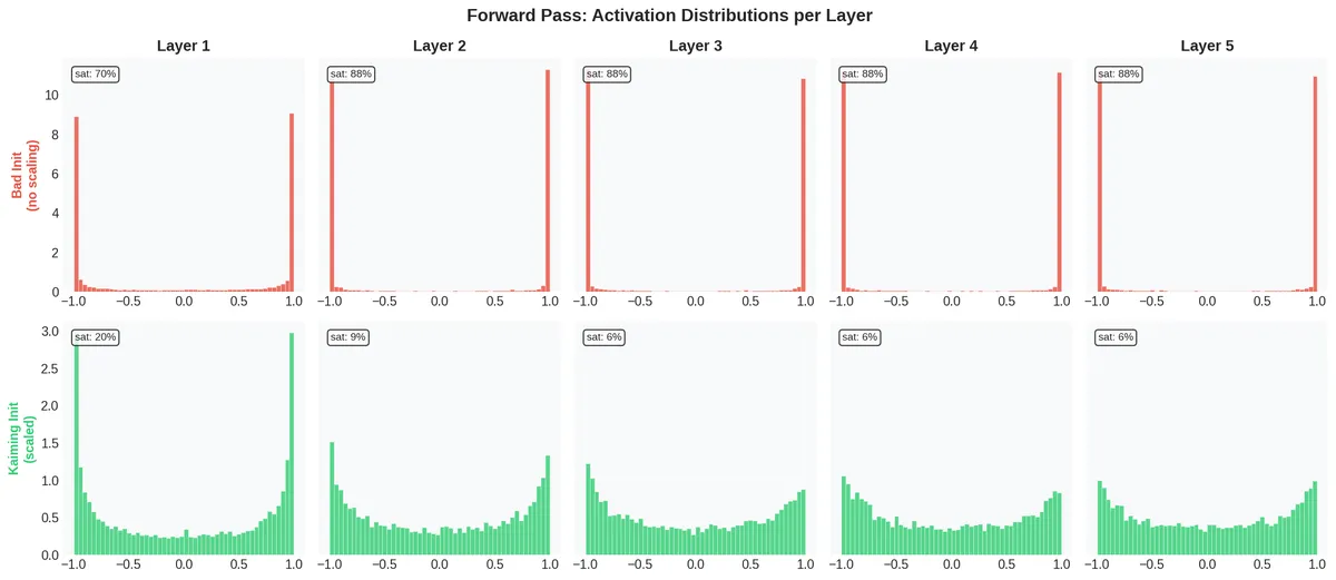
Activation distributions per layer

The top row (bad initialization) is a disaster. By Layer 2, 88% of the activations are saturated — pinned at $\pm 1$ . These are effectively dead neurons: since $\frac{d}{d x} \tanh (x) = 1 - \tanh^{2} (x)$ , any neuron with $| \tanh (x) | \approx 1$ has gradient $\approx 0$ . The network cannot learn through these neurons.

The bottom row (Kaiming initialization) keeps activations spread across the $[- 1, 1]$ range. Saturation stays around 6-9% for the deeper layers. The network is alive.

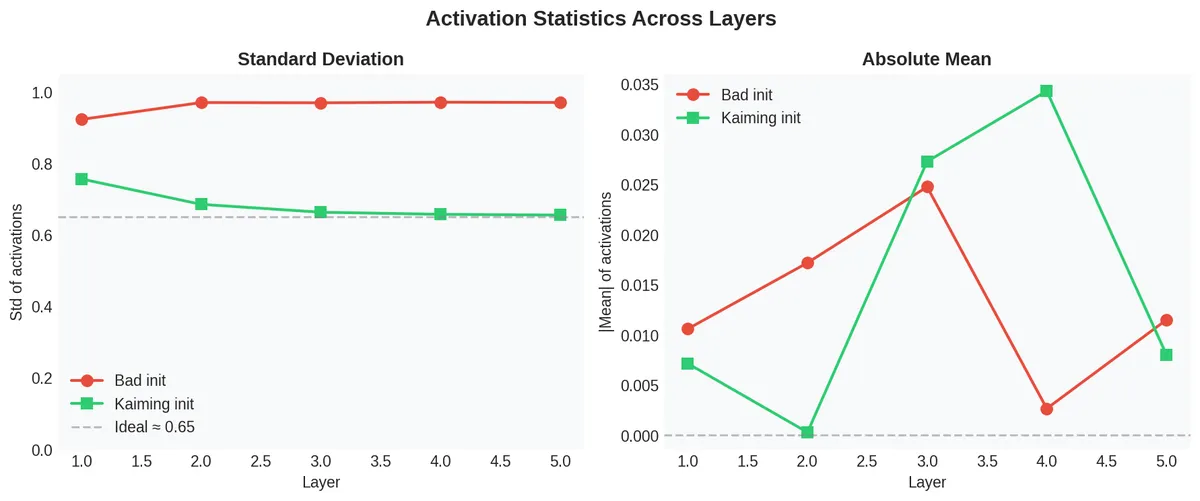
Activation statistics across layers

The left panel confirms it quantitatively: with bad init, the standard deviation of activations jumps to near 1.0 (full saturation) immediately. With Kaiming init, it stays around 0.65 — a healthy value for tanh. The right panel shows the absolute mean stays near zero in both cases, which is expected since tanh is symmetric.

The saturation problem

This bar chart makes the point directly:

Saturation per layer

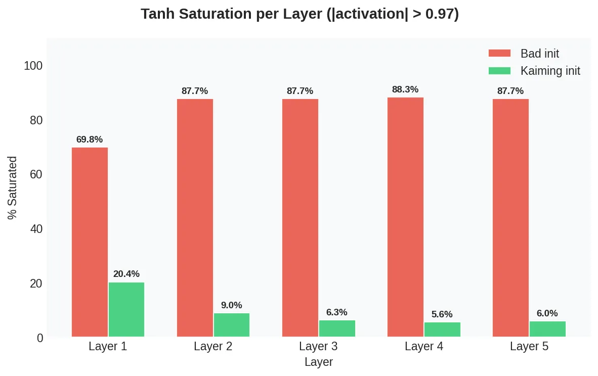
With bad initialization, the network goes from 70% saturation at Layer 1 to 88% at Layer 2, and stays there. The deeper layers are essentially not learning — gradients cannot flow back through saturated tanh units. This is the vanishing gradient problem made concrete.

Why Kaiming works

The derivation is straightforward. If the input $x$ has variance $σ_{x}^{2}$ , and weights $W$ have variance $σ_{w}^{2}$ , then the pre-activation $y = W x$ has variance $n_{in} \cdot σ_{x}^{2} \cdot σ_{w}^{2}$ . To keep $Var (y) = Var (x)$ , we need $σ_{w}^{2} = 1 / n_{in}$ .

But tanh is contractive — it reduces the spread. So we multiply by a gain to compensate:

$σ_{w} = \frac{gain}{\sqrt{n_{in}}}$

The following figure shows the three regimes on a single layer:

Why Kaiming initialization works

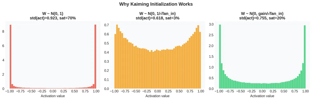
No scaling ( $σ = 1$ ): 70% saturation. Scaling by $1 / \sqrt{n}$ : only 3% saturation, but the spread is too narrow (std = 0.618) — the activations will shrink toward zero in deeper networks. Kaiming scaling (gain $\cdot 1 / \sqrt{n}$ ): 20% saturation in a single layer, but crucially this stabilizes across many layers because the gain compensates for tanh contraction.

Monitoring training: gradients and update ratios

Once the network is properly initialized, the next step is to monitor the health of gradients during training. I tracked three quantities every 100 steps:

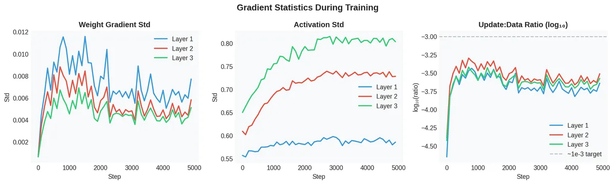
Gradient statistics during training

Weight gradient std (left): all three layers maintain non-zero gradient magnitudes throughout training. The ordering matters — Layer 1 has the largest gradients (closest to the output), Layer 3 the smallest. This is normal for a network without residual connections.

Activation std (center): the activations evolve during training but remain in a healthy range (0.55–0.80). No collapse, no explosion.

Update:data ratio (right): this is the key diagnostic. It measures how much the weights change per step relative to their current magnitude. The target is around $10^{- 3}$ — large enough to make progress, small enough not to destabilize. Our ratios are in the $10^{- 3.5}$ to $10^{- 3}$ range, which is reasonable.

The training curve

For completeness, the loss curve:

Training loss

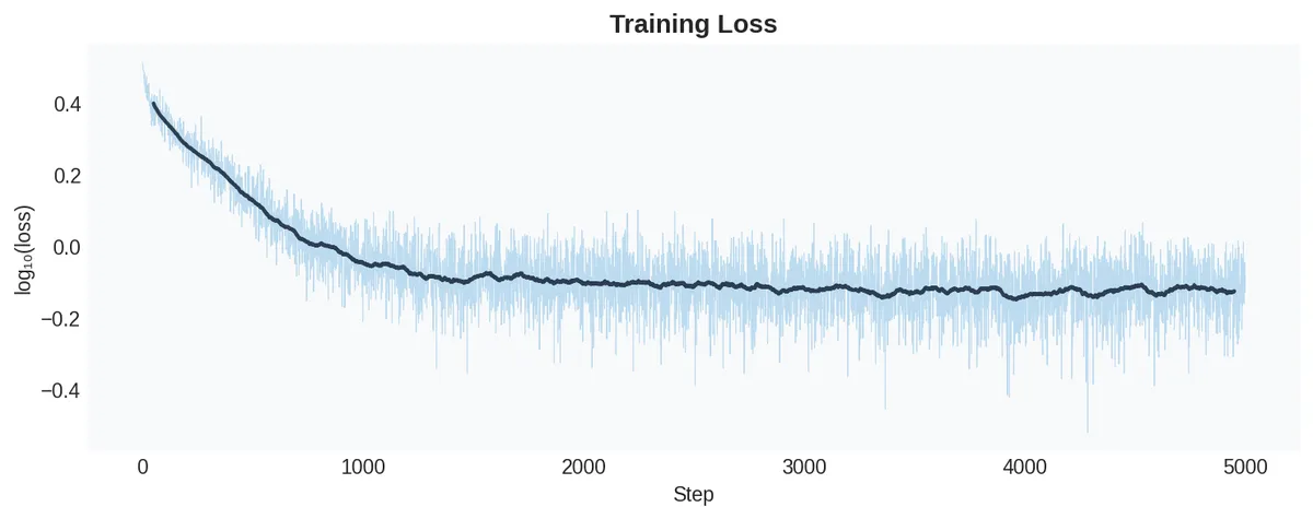
The loss drops rapidly from the expected initial value of $- \log (1 / 26) \approx 3.26$ to around $0.8$ . No hockey stick at the start — which is exactly what proper initialization gives you. The hockey stick (a large loss that suddenly drops) is a symptom of bad initialization where the network spends the first many steps just learning to produce reasonable logits.

Final weight distributions

After training, the weight matrices have the following distributions:

Final weight distributions

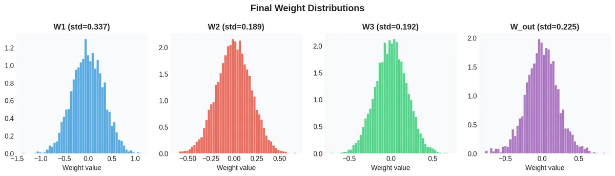
The distributions are roughly Gaussian with different standard deviations per layer, which is normal. The output layer (W_out) has learned a broader distribution than its initial $0.01$ scaling, as expected.

The complete code

Below is the full implementation — embedding, forward pass, manual backpropagation, and all diagnostics. No autograd. Every gradient is computed by hand.

import numpy as np
import matplotlib.pyplot as plt

# --- Dataset ---
names = ["emma", "olivia", "ava", ...]
chars = sorted(set(''.join(names)))
stoi = {ch: i+1 for i, ch in enumerate(chars)}
stoi['.'] = 0
itos = {i: ch for ch, i in stoi.items()}
vocab_size = len(itos)
block_size = 3

def build_dataset(word_list):
    X, Y = [], []
    for w in word_list:
        context = [0] * block_size
        for ch in w + '.':
            ix = stoi[ch]
            X.append(list(context))
            Y.append(ix)
            context = context[1:] + [ix]
    return np.array(X), np.array(Y)

# --- Network setup (Kaiming init) ---
n_embd, n_hidden, n_layers = 10, 100, 3
gain = 5.0 / 3.0

C = np.random.randn(vocab_size, n_embd) * 0.5
layers_W, layers_b = [], []
for i in range(n_layers):
    fi = n_embd * block_size if i == 0 else n_hidden
    W = np.random.randn(fi, n_hidden) * (gain / np.sqrt(fi))
    layers_W.append(W)
    layers_b.append(np.zeros(n_hidden))
W_out = np.random.randn(n_hidden, vocab_size) * 0.01
b_out = np.zeros(vocab_size)

# --- Training loop ---
for step in range(5000):
    ix = np.random.randint(0, Xtr.shape[0], 64)
    Xb, Yb = Xtr[ix], Ytr[ix]

    # Forward
    emb = C[Xb.flatten()].reshape(64, -1)
    h_list = [emb]
    for i in range(n_layers):
        pre = h_list[-1] @ layers_W[i] + layers_b[i]
        h_list.append(np.tanh(pre))
    logits = h_list[-1] @ W_out + b_out

    # Loss
    probs = softmax(logits)
    loss = -np.log(probs[np.arange(64), Yb]).mean()

    # Backward
    dlogits = probs.copy()
    dlogits[np.arange(64), Yb] -= 1
    dlogits /= 64

    dW_out = h_list[-1].T @ dlogits
    db_out = dlogits.sum(axis=0)
    dh = dlogits @ W_out.T

    for i in range(n_layers - 1, -1, -1):
        dpreact = dh * (1 - h_list[i+1]**2)  # tanh derivative
        dW = h_list[i].T @ dpreact
        db = dpreact.sum(axis=0)
        if i > 0:
            dh = dpreact @ layers_W[i].T
        # Update
        layers_W[i] -= lr * dW
        layers_b[i] -= lr * db
    W_out -= lr * dW_out
    b_out -= lr * db_out

The key line is dpreact = dh * (1 - h_list[i+1]**2). This is the tanh derivative: when h is close to $\pm 1$ , the factor $(1 - h^{2})$ is close to zero, and the gradient vanishes. This is why saturation kills learning — it is not a metaphor, it is a multiplicative zero in the chain rule.

The takeaway

The weights of a neural network are not random numbers you set once and forget. They are the initial state of a dynamical system, and that state determines whether the system can evolve (learn) or is trapped from the start. The diagnostic tools — activation histograms, gradient standard deviations, update:data ratios — are the instruments for studying this system. Without them, training is guesswork.