Scientific method for the neural network forward pass
Building neural networks implies that you are creating an entity.
Do you know it well?
Can you understand how and what this entity is learning?
This process is all about the weights, as we know. So it is really important to investigate them.
The forward pass is the model demonstrating what it knows and learned. And just like any scientific investigation, we need a method to study it. We need to observe, measure, diagnose, and then act.
This is what we will do here.
Observation
Every layer in a neural network produces an output — a list of numbers called activations. Before computing anything, we first need to collect these raw outputs and look at them.
In Karpathy's code, layer.out gives us exactly this: the activation values after each Tanh layer. This is our raw data. The starting point of any investigation.
Tanh is the activation function used in this network. It takes any number as input and outputs a value between -1 and +1. Large positive inputs produce values close to +1. Large negative inputs produce values close to -1. Inputs near zero produce outputs near zero. This is important because the shape of the Tanh function creates regions where learning can stop, as we will see.
The question here is simple: what does this entity produce when we feed it an input? We are not judging yet. We are just observing.
Measurement
Now we bring in the instruments. Three statistics tell us almost everything we need to know about the health of a layer.
Mean is the average of all activation values. Add all numbers together and divide by the count. If the mean is close to zero, the activations are balanced — roughly as many positive values as negative ones. If the mean drifts away from zero, the layer is introducing a systematic shift in the signal. For Tanh activations, we want the mean close to zero.
Standard deviation measures how spread out the values are from the mean. A small standard deviation means most values are clustered tightly together. A large standard deviation means they are spread across a wide range. In our network, this tells us how much of the Tanh range the layer is actually using. If the standard deviation is too small, the activations are all near zero and the layer is barely contributing. If it is too large, the activations are pushed to the extremes.
The ideal standard deviation for Tanh is approximately 1/√3 ≈ 0.577. At this value, the activations are spread across the full useful range of the function.
Saturation measures the percentage of activations that fall in the flat regions of Tanh, near -1 or +1. In these flat regions, the derivative of Tanh is nearly zero. The derivative is what the network uses during backpropagation to compute gradients. If the derivative is zero, the gradient is zero. If the gradient is zero, the weight does not update. The neuron stops learning.
A neuron with activation above 0.97 or below -0.97 is considered saturated. High saturation means many neurons in the layer have stopped contributing to learning.
Here is the code that collects these measurements, following Karpathy's approach:
for i, layer in enumerate(layers[:-1]):
    if isinstance(layer, Tanh):
        t = layer.out
        print(f'layer {i} ({layer.__class__.__name__}): '
              f'mean {t.mean():+.4f}, '
              f'std {t.std():.4f}, '
              f'saturated: {(t.abs() > 0.97).float().mean()*100:.2f}%')
Diagnosis
With measurements in hand, we can now interpret. I ran the forward pass on a character-level MLP — the same kind of network Karpathy builds in makemore Part 3. It has 5 hidden layers with 200 neurons each, all using Tanh activations.
I ran the same network with five different initialization strategies. The initial weights determine the network's starting state — what it "knows" before any training. Different initializations produce very different activation distributions.
The five strategies:
Naive σ=1.0 — weights sampled from a normal distribution with standard deviation 1.0. No consideration of network architecture.
Naive σ=0.2 — same approach, but with smaller standard deviation.
Xavier — scales weights by 1/√(fan_in + fan_out), where fan_in and fan_out are the number of input and output neurons. Proposed by Glorot and Bengio in 2010.
Kaiming — scales weights by gain/√(fan_in), with a gain factor of 5/3 for Tanh. Proposed by He et al. in 2015. This is what Karpathy uses.
Data-Dependent — starts with Kaiming, then calibrates each layer using the actual data statistics. A hypothesis we are testing.
Here are the activation distributions:
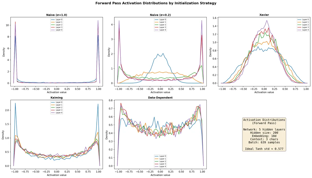
Each subplot shows the density of activation values for all five Tanh layers under one initialization.
With Naive σ=1.0, the distributions collapse to two spikes at -1 and +1. Nearly every neuron is saturated. With Naive σ=0.2, Layer 0 is concentrated near zero (underusing the range), while deeper layers progressively spread out and begin saturating — the signal grows as it propagates. Xavier produces smooth distributions that shrink in deeper layers — the signal decays. Kaiming uses more of the Tanh range but shows concentration near ±1 in Layer 0. The Data-Dependent initialization produces the most consistent distributions across all layers.
The saturation numbers make this concrete:
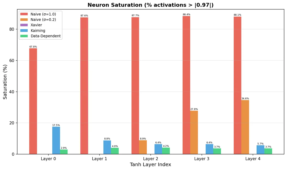
Naive σ=1.0 has 67–88% saturation across all layers. Kaiming has 17.5% saturation in Layer 0 — one in six neurons is not learning. The Data-Dependent approach keeps saturation below 4% everywhere.
All the numbers:
| Strategy | Loss | Avg Std | Std Layer 0 | Std Layer 4 | Avg Saturation |
|---|---|---|---|---|---|
| Naive (σ=1.0) | 15.5229 | 0.9611 | 0.9218 | 0.9701 | 83.9% |
| Naive (σ=0.2) | 5.4399 | 0.5851 | 0.1969 | 0.8160 | 14.3% |
| Xavier | 3.2578 | 0.3217 | 0.4007 | 0.2641 | 0.0% |
| Kaiming | 3.2571 | 0.6819 | 0.7408 | 0.6525 | 9.0% |
| Data-Dependent | 3.2523 | 0.6170 | 0.5876 | 0.6270 | 3.7% |
The most revealing plot is how the standard deviation changes from layer to layer:
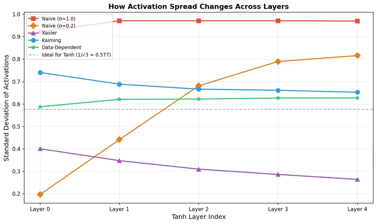
The dashed gray line is the ideal value (0.577). A good initialization should keep the standard deviation close to this line and stable across all layers.
Naive σ=1.0 is flat at ~0.97 — everything saturated. Naive σ=0.2 starts at 0.20 and climbs to 0.82 — unstable signal growth. Xavier decays from 0.40 to 0.26 — the signal is vanishing. Kaiming starts at 0.74 (above ideal) and drifts down to 0.65 — better, but not stable.
The Data-Dependent initialization starts at 0.587 — almost exactly the ideal — and stays between 0.587 and 0.627 across all five layers. The most stable signal propagation of all strategies.
Hypothesis and intervention
A scientist does not stop at diagnosis. The next step is to form a hypothesis and test it.
Xavier and Kaiming use only architectural information to set the weights: the number of input and output neurons per layer. They assume that the input to each layer has certain statistical properties (zero mean, unit variance). But this assumption can be wrong. The actual data — character embeddings, their distributions, correlations in the context window — determines what the first layer actually receives. And each subsequent layer receives the transformed output of the previous one.
This is the data-dependent initialization hypothesis: calibrating each layer's weights using the actual data statistics, not just the architecture, produces healthier activation distributions.
The procedure: start with Kaiming initialization. Run a forward pass one layer at a time. At each linear layer, measure the actual output standard deviation. Rescale the weights so the pre-activation standard deviation equals 1.0 (a value that, after Tanh, produces activations near the ideal 0.577 std). Correct the bias to center the activations at zero.
Here are the pre-activation distributions — what the Tanh function actually receives as input:
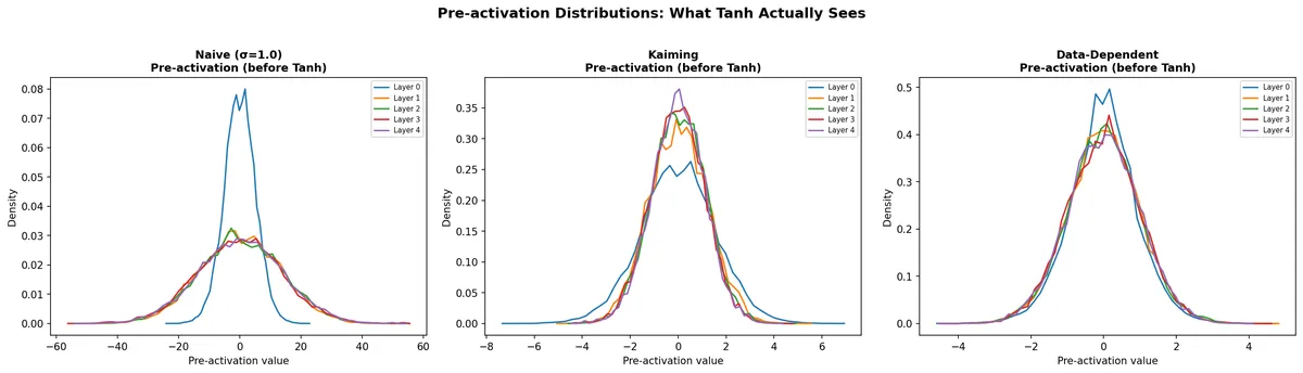
With Naive σ=1.0, pre-activations range from -60 to +60. Everything beyond ±3 is squashed to ±1 by Tanh. With Kaiming, the range is about ±6 — better, but still pushing some values into the flat zone. The Data-Dependent approach keeps pre-activations in a ±3 range, and all five layers see a similar distribution.
Conclusion
Everything measured here is at initialization — before a single step of training. The loss values (3.2523 vs 3.2571) are essentially the same. We have shown that the network starts in a healthier state. We have not shown that it learns faster or reaches a better final result.
The open questions: does this advantage survive the first hundred training steps? Does it matter more in deeper networks where signal propagation is harder? Does the calibration batch need to represent the full dataset well?
These are questions for the next experiment. What we have done here is the first half of the scientific method: observe, measure, diagnose, hypothesize. The second half — test and conclude — requires the training loop.
The forward pass gave us the evidence. Now we know where to look for understanding the learning.